Process capability indices: reading Cp and Cpk correctly

In short

Cp compares the spread of a stable process with the specification width, and it ignores where the process mean sits.
Cpk also accounts for centring, so it can never exceed Cp, and the two are equal only when the mean sits exactly midway.
Both indices mean little unless the process is first shown to be in statistical control and its data are roughly normal.

Spread and centring are two questions

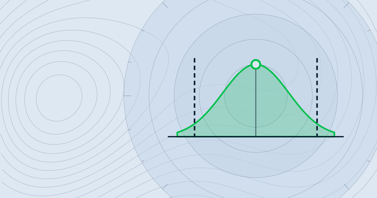
A process produces measurements, and an engineer asks two separate questions. Is the spread narrow enough to fit inside the specification window? Is the centre of the process close to the middle of that window? Cp answers only the first question. Cpk considers both.

The lower and upper specification limits, LSL and USL, come from design or customer requirements. They are not the same as control limits, which come from the process's own variation. The process mean μ and the standard deviation σ describe where the process sits and how much it varies. LSL, USL, μ and σ are the four inputs, so an index depends on both the requirement and the measured behaviour.

Formulas and what they say

Cp = (USL − LSL) / (6σ). This is the potential capability if the process were perfectly centred. The term 6σ is the width of ±3σ around the mean under normal variation.

Cpk = min[(USL − μ) / (3σ), (μ − LSL) / (3σ)]. The formula measures the distance from the mean to each limit in units of 3σ and keeps the smaller value, which is the side closer to a limit.

A Cpk of 1.00 therefore means the mean is about three standard deviations from the nearer limit. That reading assumes the distribution is approximately normal. If the distribution is skewed, the same number does not imply the same tail probability.

A hypothetical example and the centring effect

Consider a hypothetical filling process with LSL = 9.8, USL = 10.2, mean μ = 10.05 and σ = 0.05.

Cp = (10.2 − 9.8) / (6 × 0.05) = 0.4 / 0.3 = 1.33
Cpk, lower side: (10.05 − 9.8) / (3 × 0.05) = 0.25 / 0.15 = 1.67
Cpk, upper side: (10.2 − 10.05) / (3 × 0.05) = 0.15 / 0.15 = 1.00
Cpk = min(1.67, 1.00) = 1.00

Cp describes the process as if it were centred. Cpk shows that the process runs closer to the upper limit and drops to 1.00. If the mean were moved to 10.00, both sides would give 0.20 / 0.15 = 1.33, and Cpk would equal Cp. The spread did not change; only the centring did.

Conditions before the indices mean anything

An index summarises a model of the process. If the process drifts during the sample, σ may not represent its true variation, and the mean is not a stable target. Check the process with a control chart first. An index computed from a process that is out of control describes a mixture of states rather than one capability.

Normality matters as well. Skewed or multimodal data, such as a process with two operating modes, can make the normal-based interpretation misleading. Sample size also matters, and a common recommendation is 100 or more measurements. The source of σ changes the meaning too: σ from within-subgroup variation yields Cp and Cpk, while the overall σ yields Pp and Ppk. Mixing the two is a common error.

Limits and common misreadings

Target values are not part of the index. The figures 1.33 and 1.67 are often quoted, but the customer or the applicable requirement sets them. A target that suits one product may not suit another, so it should come from the requirement document rather than from a rule of thumb.

Common misreadings follow. A high Cp is taken as proof of a good process, while Cpk is low because the mean is off-centre. Control limits are confused with specification limits: a process can be in control and still out of specification, or the reverse. Cp and Cpk also do not give the fraction of output outside the limits directly; that needs a separate look at the shape of the distribution.

How to check it on your line

Begin with a control chart, such as an X-bar and R chart, to show that the mean and the spread are stable over time. Only then compute the indices. If the chart shows special-cause variation, defer the index calculation until the cause is understood.

Next, check the measurement system. Repeatability and reproducibility errors add to the observed spread, which lowers Cp and Cpk even when the process itself is good. A measurement system analysis should be done before the indices are reported. Finally, confirm the LSL and USL against the requirement document, and report the indices together with a histogram and the control chart rather than as a single number.

Frequently asked

What is the difference between Cp and Cpk?

Cp compares the process spread with the specification width and assumes perfect centring. Cpk also penalises an off-centre mean by using the nearer limit. When the mean sits exactly midway, the two are equal. If Cpk is well below Cp, centring is the first thing to examine.

Is a Cpk of 1.33 good enough?

That depends on the target set by the customer or the requirement. The value 1.33 is widely quoted, and 1.67 is often used for critical characteristics. The index is only meaningful when the process is stable and roughly normal, so check those conditions before comparing the number with any target.

Sources and further reading

Pilot steps in this guide are proposed engineering workflows. Examples do not constitute measured field performance.

Questions on this topic

What are Cp and Cpk, and how are they calculated?What is the difference between control limits and specification limits?