CUSUM and EWMA: catching small, sustained shifts

Why Shewhart charts are slow on small shifts

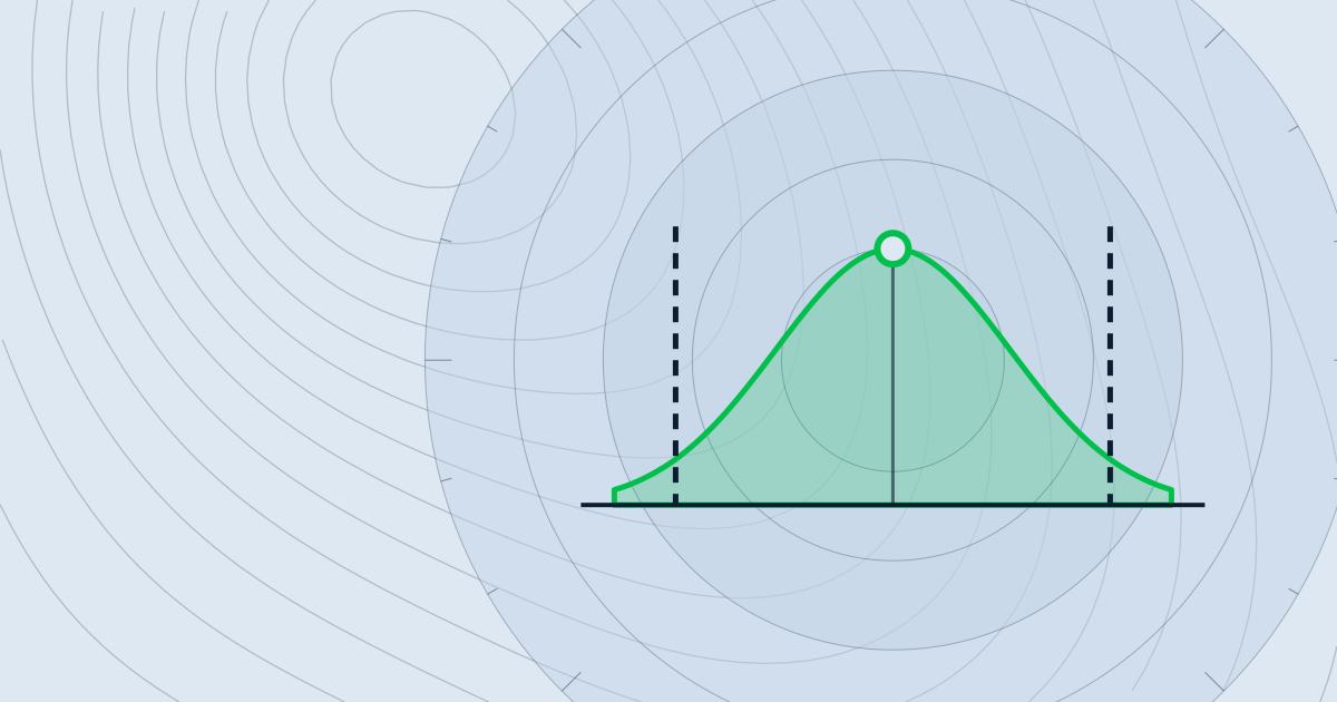
A Shewhart control chart compares each measurement with its limits. The limits are usually set at μ0 ± 3σ, where μ0 is the target mean and σ is the standard deviation estimated from a stable period. For large, sudden jumps, the chart responds quickly and simply.

However, when the process mean shifts permanently by only 0.5 to 1.5σ, a single measurement rarely crosses the limit. The signal is delayed even though the shift is real. Because every point appears inside the limits, the delay can go unnoticed. Small but sustained shifts are easier to see with CUSUM and EWMA, which accumulate or smooth past deviations.

CUSUM: accumulating deviations

CUSUM (cumulative sum) subtracts a reference value from each new measurement and adds the difference to a running total. For an upward shift, the statistic is:

S⁺_t = max(0, S⁺_(t−1) + (x_t − μ0 − k))

Here k is the slack, usually taken as 0.5σ. The reference value is μ0 + k. While measurements stay above it, the total grows; when they fall below it, the total drops toward zero and never goes below it. A signal is given when S⁺ exceeds a chosen threshold h, often set between 4σ and 5σ. A mirror statistic S⁻ works in the opposite direction for downward shifts, and both totals are monitored together.

A hypothetical CUSUM table

The example below is hypothetical: μ0 = 10, σ = 1, k = 0.5 (so the reference value is 10.5), and h = 4:

• t = 1, x = 11.0: 11.0 − 10.5 = 0.5; S⁺ = 0 + 0.5 = 0.5
• t = 2, x = 11.2: 11.2 − 10.5 = 0.7; S⁺ = 0.5 + 0.7 = 1.2
• t = 3, x = 10.9: 10.9 − 10.5 = 0.4; S⁺ = 1.2 + 0.4 = 1.6
• t = 4, x = 11.4: 11.4 − 10.5 = 0.9; S⁺ = 1.6 + 0.9 = 2.5
• t = 5, x = 11.1: 11.1 − 10.5 = 0.6; S⁺ = 2.5 + 0.6 = 3.1
• t = 6, x = 11.6: 11.6 − 10.5 = 1.1; S⁺ = 3.1 + 1.1 = 4.2, which exceeds h = 4

The six values average 11.2, about 1.2σ above μ0. None exceeds the upper Shewhart limit of 13.0, but CUSUM signals at the sixth measurement. S⁻ stays at zero, since it grows only when a value falls below 9.5, and none does.

EWMA: exponentially weighted average

EWMA blends each new measurement with the previous smoothed value:

z_t = λ·x_t + (1−λ)·z_(t−1)

Here 0 < λ ≤ 1 is a weight. A smaller λ gives more weight to older values, which makes the chart smoother and slower to react. Typical values of λ lie between 0.05 and 0.25. The control limits are μ0 ± L·σ·√(λ/(2−λ)·(1−(1−λ)^(2t))), and L is commonly chosen between 2.7 and 3.

Hypothetical example: λ = 0.1 and L = 2.7. As time passes, the bracketed term approaches 1, and the limits approach μ0 ± 2.7·σ·√(0.1 / 1.9). Evaluating the root gives √(0.1 / 1.9) ≈ 0.229, so the limits settle at about μ0 ± 0.62σ. For the EWMA statistic, these limits are much tighter than the ±3σ Shewhart limits, so a small shift can become visible sooner.

Autocorrelation and false alarms

CUSUM and EWMA assume that measurements are independent. If consecutive values are related, so that one reading resembles the previous one, deviations can accumulate without any real shift, and false alarms increase. The effect is strongest in data streams where successive samples are taken very close together. In that case, monitoring the residuals of a model fitted to the raw values, rather than the raw values themselves, may be worth considering.

Another risk is the estimate of σ. It should come from a stable in-control period. A σ taken from a window that includes maintenance, a product change or a shift pattern will make the limits too wide or too narrow. State in the report which period the σ was taken from.

Choosing parameters and starting

Begin by defining the smallest shift you want to catch. If the shift to detect is δσ, a common starting point is to set k at about δ/2; for a 1σ shift, k = 0.5σ. Then set h according to the false-alarm rate you can accept. That rate is often expressed as the average run length (ARL): the average number of measurements before a false signal occurs in an in-control process. A larger ARL means false alarms are rarer, but the delay in seeing a real shift may grow.

To start, estimate σ from a stable period, compare Shewhart, CUSUM and EWMA results on the same data, and record whether each signal corresponds to a real process change.

Frequently asked