Kalman filtering: a smoothed health indicator from a noisy sensor

In short

A Kalman filter estimates a hidden state recursively from noisy measurements, weighing the model prediction against each new reading.
The gain K = P / (P + R) balances prediction uncertainty against measurement noise, so a larger R makes each reading count for less.
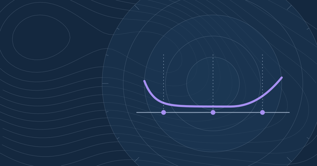
Using level and slope as states gives a smoothed health indicator together with its rate, which can feed a remaining-life estimate.

Estimating a state from noisy readings

A sensor rarely reports the quantity you care about directly. A vibration accelerometer adds measurement noise and short transient spikes on top of the true degradation level. A Kalman filter treats the measured value as a noisy view of a hidden state, and it updates its estimate of that state with every new reading.

Each cycle has two steps. In the predict step, the previous state and its uncertainty are carried forward to the next time step using a model. In the update step, the difference between the new measurement and the prediction, called the innovation, is used to pull the estimate toward the measurement. Only the latest state and its variance are stored, so memory use does not grow with the length of the history.

The gain: trusting the model or the sensor

The gain K sets how much the innovation changes the estimate. For a scalar state, with P the prediction variance and R the measurement noise variance, K = P / (P + R). The estimate becomes the prediction plus K times the innovation.

The intuition is straightforward. If P is small, the prediction is confident, K is small, and the filter leans on its model. If R is small, the sensor is precise, K approaches one, and the filter follows the measurement. The process noise Q describes how much the true state may change between steps. In a simple random-walk model, the predict step adds Q to P. A larger Q keeps the uncertainty from shrinking, which stops K from falling too far. The ratio of Q to R sets how quickly the filter tracks the data.

A hypothetical scalar example

Suppose the prediction is 10 with variance P = 4, and a hypothetical measurement of 12 arrives with noise variance R = 4.

K = P / (P + R) = 4 / (4 + 4) = 0.5
Estimate = 10 + 0.5 × (12 − 10) = 11
New variance = (1 − K) × P = 0.5 × 4 = 2

The estimate lands halfway between prediction and measurement, and the variance halves. If the sensor noise were R = 1 instead, K = 4 / (4 + 1) = 0.8 and the estimate would be 10 + 0.8 × 2 = 11.6, so the sensor would be trusted much more. These numbers are for comparison only. Real P and R values must come from tests on your own sensor and model.

Level and slope for degradation

Degradation signals often carry a trend, and a filter with only one state lags behind it. A local linear trend model puts both the level and the slope into the state vector. The filter then produces a smoothed health indicator and an estimate of how fast that indicator is changing.

The slope is the main input to a remaining-life estimate. The time to threshold can be computed from the current level, the threshold and the slope. The uncertainty of the slope comes from the covariance matrix of the state. When the slope is uncertain, the remaining-life band is wide. If the data do not yet show a clear trend, that wide band is an honest result and is more useful than a single precise date.

Limits and outlier handling

The standard Kalman filter assumes a linear model and Gaussian noise. Real degradation is often nonlinear, and sensor noise is frequently heavy-tailed, with occasional spikes. In those cases the filter is an approximation, and its uncertainty band should be read as conditional on the model.

Outliers need explicit handling. A single bad reading, such as one from a loose connector, can pull the estimate far off. A common safeguard is to monitor the normalised innovation and to gate out measurements whose innovation is implausibly large. Irregular sampling is another limit: the state transition depends on the time step, so the model must use the actual elapsed time rather than assuming a fixed interval.

How to start on your data

Begin by recording the sensor while the machine is at standstill. The noise in that record gives a first estimate of R. Do not set R by eye from a plot of the running signal, because that mixes measurement noise with real vibration.

Next, choose Q by testing against a known event, such as a documented level change after a repair or a recorded fault. If the filter responds too late, Q is probably too small; if it follows every spike, Q is probably too large or R too small. Plot the raw signal and the filtered health indicator together over historical data, and record the lag, the false excursions and how outliers were handled before anyone relies on the output.

Frequently asked

How does a Kalman filter differ from a moving average?

A moving average smooths over a fixed window and does not model measurement uncertainty. Exponential smoothing is a simple form with a fixed gain. A Kalman filter changes its gain at each step according to the uncertainty, and it can estimate hidden states such as the slope.

When does a Kalman filter mislead?

It misleads when the model is wrong. A linear model applied to a nonlinear degradation gives lag or a false trend. Setting R too small or Q too large lets noise back into the estimate. Check the output against known events and historical failure records before trusting it.

Sources and further reading

Pilot steps in this guide are proposed engineering workflows. Examples do not constitute measured field performance.

Questions on this topic

Why is RUL estimated as a range instead of a single number?What is a Kalman filter and how does it work on noisy sensor data?